Drawing bugs with Python and Pillow
Last weekend I spent some time playing with a fun side project that I had been thinking about for a while. I remember as a kid, I think it was in a Scientific American issue that someone described a computer program to generate insect-looking drawings, which evolve over time into increasingly weird looking critters. The point was to demonstrate the ease with which evolution can produce vastly different living beings, thus explaining the immense diversity of life on Earth. But all I remember thinking is how interesting those little bugs looked.
So I decided to repeat the feat and in the process teach myself some technologies I had been meaning to learn for a while:
- Pillow is one of the most popular image drawing kits for Python. It’s based on the venerable PIL and while it has its quirks, it’s handy for image processing as well as for synthetic drawing.
- Flask is a minimalistic web framework that is surprisingly fun to work with. Compared to Django, my go-to choice, Flask is much faster to get started with, although it doesn’t provide as many built-in niceties.
- Lambda is the serverless computing platform provided by AWS. It’s handy to deploy small projects to the web without having to commit to big server expenses, because the app runs completely on demand, and does not just sit idle when there’s no use.
- Vue.js is a JavaScript framework that lets you add interactivity to your frontend without adding too much complexity. I see it as a good replacement for jQuery that doesn’t impose as much burden as Angular or React. Perfect for this toy project.
In this post, however, I will only talk about the drawing part. Using Pillow to draw basic shapes, organizing your code logically, and allowing for future work.
Let’s draw something⌗
Before we get into the gory details, it’s probably a good idea to show how some basic shapes can be drawn using Python and Pillow.
I recommend that you take a look at the tutorial in the official documentation, but if you want to dive right in, create a file called rectangles.py and add the following contents:
import random
from PIL import Image, ImageDraw

width, height = 256, 256  # A square image
background = (0, 0, 0, 0)  # Transparent background (RGBa format)
im = Image.new('RGBA', (width, height), background)  # Get an Image object
draw = ImageDraw.Draw(im)  # An ImageDraw handler for drawing on the image

# Draw random rectangles, with random colors too
for _ in range(30):
    color = tuple(random.randint(127, 255) for _ in range(3))  # Not too dark
    corners = tuple(random.randint(0, 255) for _ in range(4))  # (x1, y1, x2, y2)
    line_width = random.randint(1, 10)
    draw.rectangle(corners, outline=color, width=line_width)

im.save('rectangles.png')
If you follow along those 12 lines, you can see that what we do is:
- Create a square, blank
Imageobject and anImageDrawobject to draw on it - Randomly specify 30 rectangular shapes, with random RGB colors and line widths
- Save the image as a .png file
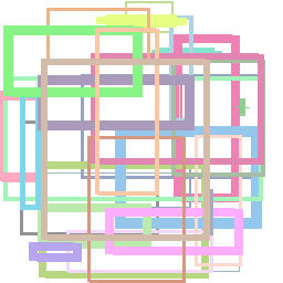
Now, run the script entering python3 rectangles.py in the terminal, and inspect the resulting image in rectangles.png. If you didn’t run into any problems, you will see something similar to the following image:
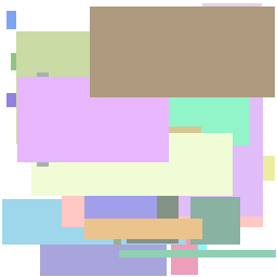
Play with the code and inspect the many options available. For example, you can pass a fill parameter which indicates the color for the interior of the shape, instead of just the outline. You may get something like this instead:
If you look at the documentation, you’ll see many other drawing functions, but for this project we will only care for two:
- draw.ellipse() to draw circles. The parameters are not ideal because you need to compute the enclosing box, instead of going by center and radius. Some simple geometry will go a long way here.
- draw.line() to draw the legs. By providing a width, you actually draw solid rectangles, and this is more convenient than the
rectangle()method because the orientation arbitrary.
Now that you know how to draw lines, rectangles and ellipses, we can move on to doing something more complicated, and more fun.
Note: If you haven’t done so already, you may have to install
Pillowon your computer. Something likepip3 install Pillow Imageworks for me, but your system can be different.
Drawing something more complex⌗
When you prepare to draw some complex shapes, you can start writing the drawing code with hardcoded parameters. But pretty quickly you run into the problem of intermingling your logic and display code. This is a common pattern in computer science, and it’s better handled by separating the concepts of structure and presentation. For example, when you write a website, it’s advisable to use HTML for markup (the structure), and leave the display details to the CSS styling (the presentation).
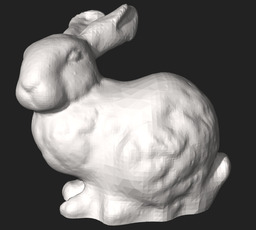
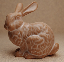
In computer graphics this is seen time and time again. You may have seen various renderings of the Stanford bunny (3D model used with permission from Stanford Computer Graphics Laboratory). They all spring from the same shape definition (the structure), but using various techniques, you can achieve substantially different results:
In our toy project we will follow the same principle of separating the definition of what we want to draw from the process of actually drawing it.
Shape specification and rendering process⌗
When we set to draw a bug, the first think to think about is what does a bug look like. In our imaginary universe, a bug has a torso, a head, a tail and an arbitrary number of leg pairs. An actual definition for a bug with 6 legs (a bona fide insect!) could look something like this:
sample_bug = {
    'fill': (80, 80, 0),  # Color of the bug
    'thickness': 20,  # Base thickness of the torso
    'head': {
        'sz': 2,  # Head size as a multiplier over the thickness
    },
    'tail': {
        'segs': [.06, .04, .02],  # Segments that make up the tail
    },
    'legs': [
        # Each leg is given the spacing from the previous one, number of segments,
        # total length, and width multiplier with respect to the torso
        {'gap': 1, 'segs': 3, 'len': .25, 'w_mult': .4},
        {'gap': 3, 'segs': 4, 'len': .19, 'w_mult': .5},
        {'gap': 2, 'segs': 3, 'len': .15, 'w_mult': .4},
        {'gap': 2, },  # Last segment is just for spacing
    ],
}
Once we have a basic shape definition, we can start thinking about how to display it. This is called the rendering process. We take the definition of the shape and turn it into the lines, rectangles and ellipses that make our beloved bug.
Note: In a more complete solution, we would have an intermediate step where we apply a series of geometric transformations to the model (rotating, scaling, translating and shearing its components) in order to compute the actual coordinates of each part of the bug before rendering. Since this is a quick and dirty project, we have combined both steps into one. In a future iteration we may have to separate them to reduce complexity.
At this point we are able to render the bug by essentially iterating over its various components (torso, head, tail, legs) and drawing each one in relation to the previous one. We start with the torso, keeping track of the top-bottom coordinates, as well as its length, and use those values to compute the starting point of each pair of legs, the head and the tail segments.
The code to render the entire bug is perhaps too long (and currently overcomplicated, to be honest) but as a sample here’s the code to draw leg, starting form the position of the joint, and moving outward. Each segment of the leg shrinks by a constant factor, and is also slightly rotated toward one of the ends of the bug (head or tail).
def draw_leg(draw, start, base_thickness, width_factor, segment_len, num_segments, angle, fill, direction=1):
    # Param `direction` is 1 for right, -1 for left
    thickness = base_thickness*width_factor
    angle_ref = angle
    for x in range(num_segments):
        diff = rotate((direction*segment_len, 0), direction*angle)
        end = translate(start, diff)
        line = (start[0], start[1], end[0], end[1])
        draw.line(line, fill=fill, width=int(thickness))
        start = end
        thickness *= width_factor
        segment_len /= GOLDEN_RATIO
        angle += angle_ref
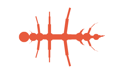
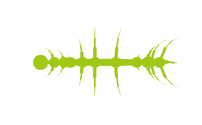
We repeat this for each leg, passing direction=1 on the right side and direction=-1 on the left, and we have a bug somewhat like this one, which we have rotated for a better fit in this document:
Perhaps the only part that requires a small explanation is the rotation function. But the math for geometric transformations is often expressed in the form of matrix multiplications. Specifically, the 2D rotation matrix involves computing the sine and cosine of the rotation angle. We then multiply it (i.e. apply its inner product) by the coordinates of the point we want to transform, and the result is the location of the rotated point. In a simplified form, it’s as follows:
def rotate(point, radians):
    cos = math.cos(radians)
    sin = math.sin(radians)
    return (cos*point[0] - sin*point[1], sin*point[0] + cos*point[1])
Perhaps I will to explain this and other transformations in more detail in the future.
Evolving our creatures⌗
What we have now is the rendering of a predefined shape. To make things more interesting, we can apply randomized evolution process to alter the specification in an incremental way. In other words, we simulate the natural process of evolution by mutating the various components such as lengths, widths, number of legs and segments, and color.
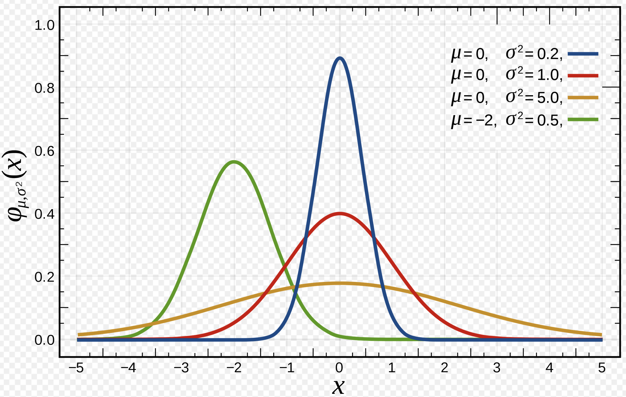
To simulate the natural process we use a Gaussian random process, which arises naturally in many aspects of life. In short, the resulting value is likely similar to the original, and less likely to be very different. This is, for example, the reason why children of tall parents tend to be tall as well, but not necessarily the same exact height. Sometimes this is also known as the normal distribution.
Again, the code for the complete randomization is probably too much for this already long blog post, but here is the code for the leg randomization:
def randomize_leg(leg):
    leg['gap'] = max(0, random.gauss(leg['gap'], .2))
    if 'segs' in leg:
        leg['segs'] = max(2, round(random.gauss(leg['segs'], 1)))
        leg['len'] = min(.5, max(0.01, random.gauss(leg['len'], .005)))
        leg['w_mult'] = max(0.01, random.gauss(leg['w_mult'], .01))
Apply this or something similar to this to every component of the bug specification, then repeat a few times, and pretty soon you begin to see some pretty interesting shapes.
Future work⌗
That’s all for now! We will revisit this topic from other points of view, including the different technologies involved in the development and deployment of the bug evolution system. These are some ideas for the future:
- Bugs are not nearly as fun as… creepy moving bugs!
- You can antialias your image by rendering at a larger size than your desired output, then scaling down with
resize()andfilter=Image.ANTIALIAS. This technique is called supersampling, and we can discuss it another day. - Serve the images with more context so that they’re easily saved on your computer with a nice name
If you found this interesting, or if you have any comments or questions, drop me a line. My Twitter handle is at the top of this page!